Cloud Motion Vector System for Solar Power Forecasting

The world is moving towards a more sustainable source of energy like solar. However, natural energy sources are susceptible to weather conditions such as temperature and cloud cover. This means that energy supply can fluctuate below what the actual demand is. To make sure the demand is always met, it is important to provide alternate backup energy sources like batteries and motors to supplement the remaining demand. Since this switch is not instantaneous, it is also important to forecast the power output of the solar power plant. The project proposes a system which detects that a cloud cover is coming and how much power reduction is produced due to this cover.

System Overview

This project is part of a bigger network of sensors to forecast solar irradiation and ultimately, solar power output from a solar power plant or a photovoltaic (PV) system. One of the components of the network is the Cloud Motion Vector (CMV) Sensor System which uses a cluster of ambient light sensors to determine a cloud shadow’s speed and direction. From here, the data collected is fed into the PV system model where the irradiation and time-of-arrival are derived.

The CMV System consists of the following:

• BeagleBone Black rev.C
• TIVA-C microcontroller (TMC4C123GXL)
• 9x TSL2561 – ambient light sensors

The TIVA-C plus the TSL2561s are grouped together as the sensor cluster. The cluster gathers ambient light data every 150 milliseconds. Then the data is transferred to the BeagleBone Black through USB-UART. The BeagleBone Black saves the data as a CSV file and transmits it to an online server on
ThingSpeak.com
with the help of a Python script.

MATLAB scripts are used to convert the CSV data to irradiance with respect to a pyranometer, an actual irradiance sensor. This keeps the cost low as the irradiance sensors like the Apogee SP-110 cost around $200, while the TSL2561 is can go as low as $1.10. Using the TIVA-C is really handy here because it has
three
I2C buses that can be used. This means that multiple devices with the same slave address can be utilized without additional hardware (ie. i2c multiplexer). The cloud motion speed and direction is extracted using other MATLAB scripts. Finally, the these outputs can be used on a Simulink model of the PV system to forecast the power output.

Note: This is prototype uses MATLAB scripts

for convenience, but the computations can be done using

Python.

Algorithms

To determine the cloud motion speed and direction, the following algorithms are utilized:

• Linear Cloud Edge Method
• Gradient Matrix Method
• Peak Matching Method

The
Linear Cloud Edge Method
is detailed by Bosch etal. (
http://maeresearch.ucsd.edu/kleissl/pubs/BoschKleisslSE2013_CloudSpeed.pdf
). The method extracts the cloud speed and direction by a triplet of sensors. The data collected from these triplet is manipulated using rudimentary trigonometric functions. The cloud shadow speed can be expressed as:

The equation below is the angle:

And can be simplified for sensors that are perpendicular to each other:

One important thing to take note is the need of two cloud events to take place within a small time interval.

The
Gradient

Matrix

Method
is based on edge detection used on image analysis. Here the data gathered from the system is arranged into a 3×3 image/matrix and is processed to find the "edge" of the cloud shadow. The Sobel filter or kernel is convolved with the 3×3 matrix.

The convolution of the matrix and kernel yields the magnitude Gx and Gy. From here we can obtain the angle:

The
Peak Matching Method
uses the relationship of speed is equal to distance over time:

For a pair of sensors A and B, the time lag between the peaks and the valleys for the pair (
t_AB
) is used to calculate the speed for that pair. The speed from several sensor pairs are used, with respect to the direction found in the Gradient Matrix Method, to determine the estimated cloud shadow speed.

The Build

Now that the theory is out of the way, time to dig into the build. The TIVA-C is hooked up to 9 TSL2561 sensors as seen on the schematic below.

The TSL2561’s slave address can be changed by tying the
Addr
pin to
LOW
,
HIGH
, or
FLOAT.
Since the there are 3 separate I2C buses, the slave addresses do not conflict.

The code is programmed with Energia. Different modes are set but mainly the csvCollect() or Function 1 is used. Once the code is uploaded into the board, it’s ready to accept a serial command from the USB-UART.

The BeagleBone Black is connected to the TIVA-C using a USB-Ethernet extender. This can be replaced with a really long USB cord but those get expensive so I went with this configuration (the university had spare cat5 cables lying around
😛
). The BeagleBone Black runs a BASH script called
CMV.sh
that runs every morning (before the sun rises) which is 5am PST for Nevada. This can be configured by calling
crontab
:

crontab -e [username]

and adding the lines to the end of the file

0 12 * * * /home/ubuntu/CMV.sh > /home/ubuntu/cron.log 2>&1

This basically says at
12am UTC
(equal to 5am PST)run
CMV.sh
and put all terminal outputs to a file called
cron.log
.
2>&1

says to redirect
stderr
to the value
stdout
is set as.

Within the
CMV.sh
, 3 functions with python scripts are referenced:

• collectData
  – append received UART into a CSV file with a timestamp
• sendToThingspeak
  – send last line of data on the CSV file for visualization to ThingSpeak.com
• saveData
  – save a copy of the CSV file and rename it using date timestamp

Note:

Make sure to set the

proper file permissions using
chmod

command.

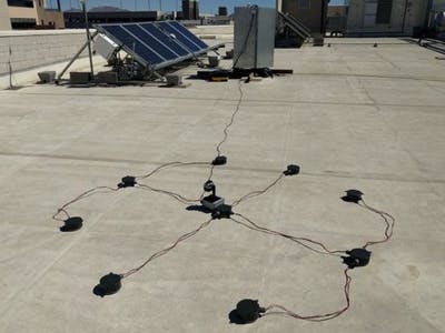
The components then go into their respective enclosures. Here’s a mini-gallery. :]

Experimental Setup

The CMV system is placed on the rooftop of the my university’s engineering building. Synthetic and actual cloud data is collected for a few days. For the synthetic data, an artificial cloud aka cardboard is passed over the CMV sensor. The directions and speed are verified using an attached gyro and recorded time.

The first row is the raw data illuminance (lux) data taken from the CMV sensor. The second row is the processed irradiance data; normalized and stuff. The last row shows the direction of the cloud shadow as a polar histogram. The coordinate with the most occurrence equates to the estimated direction.

The same thing is done for the actual cloud data, where the sensor is left on the rooftop to capture real cloud shadow events. Sample results can be seen below.

PV System Model

After finding the cloud motion vector, it time to plug our transformed sensor data into the PV System Model. This definitely varies according to the size and configuration of the site. In my case, the university has a 12kW PV system. It’s not a one-to-one model, but it meets the general requirements to run a simulation.

The figure above shows a simplified model of the PV System and sample run of the simulation. The one below is a more elaborate model with a simulated power output based on real irradiance values taken from the CMV Sensor System.

The figure above shows the progression of our data starting from the raw illuminance output that we get from the CMV Sensor System. We have the converted irradiance data, which gets fed as input of the the PV System model. The final graph is the PV System Power output in kilowatts.

The Forecast

According to Nomura etal. (
https://aip.scitation.org/doi/pdf/10.1063/1.4974806
), with the angle and speed of the cloud shadow known to us plus the distance of PV site and its angle of separation, we can do a time-of-arrival forecast. Looking at the UNLV Microgrid PV System, we can find distance to be around half a kilometer (
d
) and the
theta
= 151º. So let’s say that a cloud shadow has been detected by our sensor with a speed of
v
= 6 m/s and direction heading
a
= 120º, we can expect the cloud shadow to hit the PV System in 97.2 seconds.

Clouds Are Complicated

Of course, clouds aren’t simple creatures. They morph and change in shape, size, and height depending on the temperature, humidity, and other conditions. But the assumption is that the cloud undergoes little change from the CMV Sensor System to the PV System. This is due to the sensor system being sufficiently close to the PV System under test.

Now imagine having the the CMV Sensor System spread throughout the city. It will be like having a large ground camera taking a real-time video (in irradiance) of the clouds as they move about. These "images" can then be translated easily into power output if you have models for the PV systems within the city. This idea should bring us closer to more reliable solar power plants and a step closer to a smart city.